The Aggregate Supply curve graphs the total amount of output produced at various price levels.
The short run Aggregate Supply Curve is upward sloping.
The long run Aggregate Supply Curve is vertical.
|
|
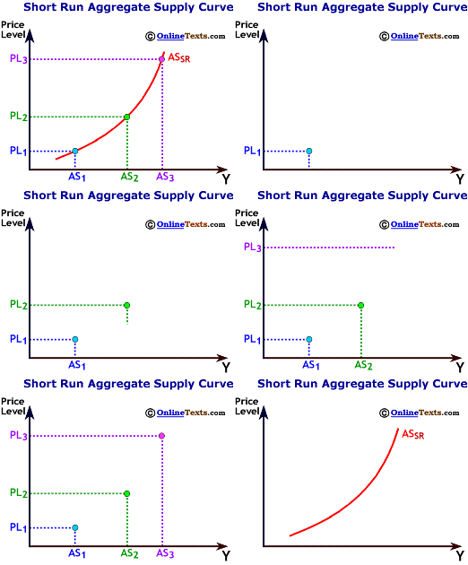
The Aggregate Supply curve graphs the total amount of output (Y) produced at various price levels. A significant difference exists between the short-run Aggregate Supply curve and the long-run Aggregate Supply curve. In the short run the Aggregate Supply curve is upward sloping. In the long run the Aggregate Supply curve is vertical.
In the context of the Aggregate Supply curve, the short run is a time period in which the costs of production--wages, raw materials, energy, and so on--are held constant; only output prices vary. When prices rise, the level of Aggregate Supply also rises because firms seek to take advantage of the profit opportunities. A firm's profit is the difference between its revenues and costs over a given time period, say one year. Suppose that a firm produces picture frames and it uses only one input, labor. Each picture frame requires one labor hour to produce, and wages are $8 per hour. The firm sells each picture frame for $10 so the profit per picture frame is $2 ($10 - $8). If the firm sells 2,000 picture frames in the first year, its total profit is $4,000 (2,000 x $2). In the second year, the firm increases the price per picture frame to $11. By assumption, wages are unchanged at $8 per hour. The firm's profit per frame produced is $3. The chance for the firm to increase its profits provides an incentive for the firm to increase production. By producing and selling 2,500 picture frames in the second year, the firm's profits rise to $7,500 (2,500 x $3). An increase in the price level, therefore, leads to a short run increase in Aggregate Supply. The Figure labeled "Short Run Aggregate Supply Curve" is upward sloping, which illustrates the positive relationship between the price level and Aggregate Supply.
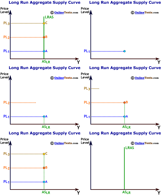
We define the long run as a time period in which all prices and costs are variable. An increase in the price level will have no impact on Aggregate Supply in the long run because all firms' costs (e.g. wages and resource costs) will rise proportionally with the price level. Recall that the picture frame company increased profits by increasing the price of picture frames from $10 to $11. Over time, workers adjust their wage demands upward because goods and services are more expensive and because good workers are harder to find as employment rises with the level of production. Suppose that workers increase their wage demands to $9 per hour. Now the firm earns the same $2 profit per frame as it did before the price level increase and the level of output returns to 2,000, the same level of production as in the first year. In the long run, the Aggregate Supply curve is vertical as illustrated in the Figure labeled "Long Run Aggregate Supply Curve." When resources such as labor and capital are fully employed, the economy's production is at the potential level of output, Yp. When the economy is on the Long Run Aggregate Supply curve, GDP is equal to potential output.
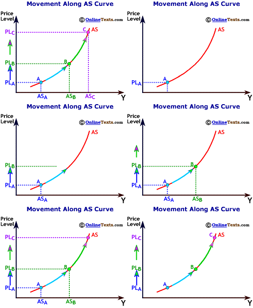
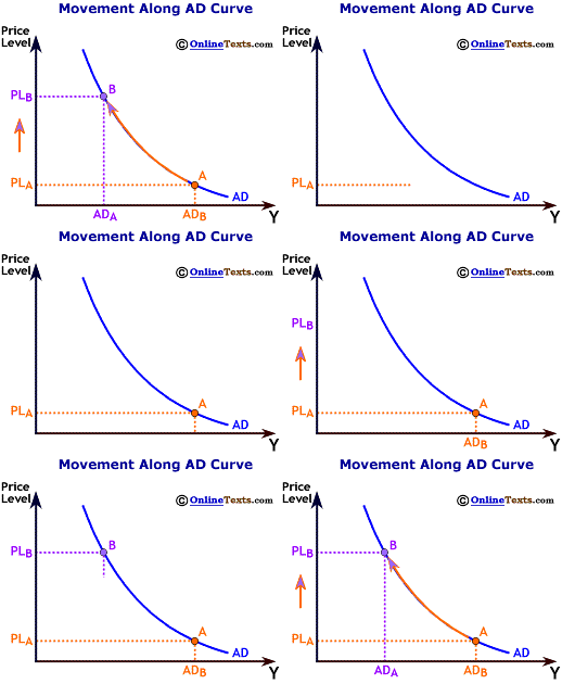
Short-run Aggregate Supply is influenced by a number of factors. One factor that we have discussed is a change in the price level. When the price level changes but resource costs are held constant, there is a movement along the Aggregate Supply curve. The figure titled "Movement Along AS Curve" graphs this scenario. As the price level rises from PLA to PLB, Aggregate Supply rises from ASA to ASB.
A change in any factor other than a change in the price level that changes the level of Aggregate Supply shifts the Aggregate Supply curve. Three nonprice factors that shift the Aggregate Supply curve are changes in resource costs, technology and inflation expectations.
An increase in the cost of a resource will shift the Aggregate Supply curve to the left. Resource costs include wages, capital, energy, and so on. Recall that the picture frame firm increased production when it had a chance to earn higher profits and reduced production when wages increased, reducing profits. If resource costs increase a firm's incentive to produce decreases as its profits decline. When oil costs increase, for example, profits decrease because energy costs increase as utility bills and fuel expenses rise. For a given price level, firms respond to rising resource costs by decreasing Aggregate Supply.
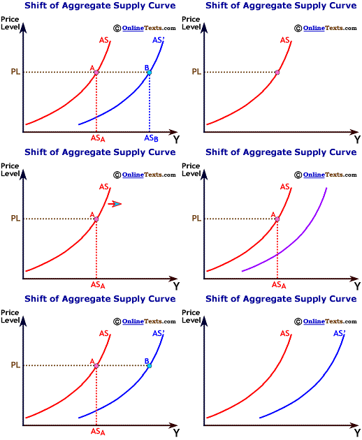 A second factor that shifts the Aggregate Supply curve is a change in technology. As the Figure titled "Shift of Aggregate Supply Curve" illustrates, an increase in technology shifts the Aggregate Supply curve to the right. Technological progress influences the economy in a variety of ways. One channel is the introduction of entirely new goods and services. Just a few years ago an on-line textbook was not possible. Advances in the Internet, however, have enabled information to be delivered in a new way. Another way that technology influences the economy is through quality enhancements of products. In contrast to automobiles produced in the 1970s, today's cars are more dependable thanks to fuel injection systems and other automated components. Newer automobiles are also more fuel-efficient, and they have air bags and other safety features that older cars lack. A third way that technology is integrated into the economy is through cost-reducing innovations. The same product can be produced at a lower cost. First-generation computers used to take up areas the size of football fields. Today some hand-held calculators are just as powerful as those computer but the cost of producing a calculator is far less than the cost of producing an old-generation computer. Given the price level, cost-reducing technological advancements allow firms to increase production and boost profits.
Changes in inflation expectations also shift the Aggregate Supply curve. If workers believe that inflation will increase in the future, they will bid up wages to compensate for the coming inflation. For a given price level, the increase in wages shifts the Aggregate Supply curve to the left.
Equilibrium in the macroeconomic sense occurs when the demand for final goods and services equals the supply of final goods and services. A short-run equilibrium, however, differs from a long-run equilibrium because in the long run the economy must be producing at the potential level of output so that all factors of production are fully employed.
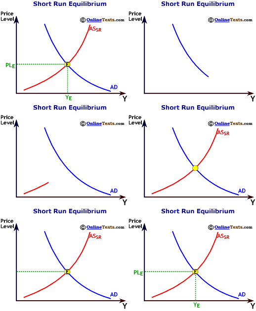 The short-run equilibrium occurs where the Aggregate Demand curve crosses the short-run Aggregate Supply curve. The intersection of Aggregate Demand and Aggregate Supply in the figure labeled "Short Run Equilibrium" determines both the price level and the equilibrium level of GDP in the economy. The level of output can be above or below potential output. For example, suppose that the economy produces $9 trillion of goods and services in the year 2005 and potential output is $8.5 trillion. As long as the demand for final goods and services is also $9 trillion, the economy is at a short-run equilibrium. Because supply and demand are equal, firms do not overproduce, which would lead to an unintended accumulation of inventories. Nor do firms underproduce, which would lead to an unintended depletion of inventories.
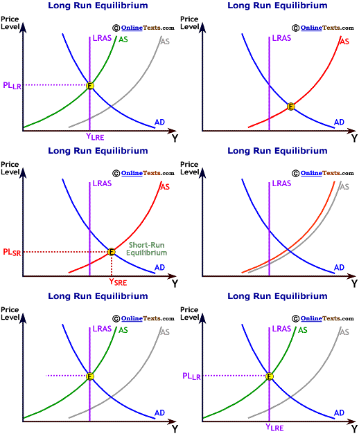 The long-run equilibrium can only occur where the Aggregate Demand curve crosses the vertical Long Run Aggregate Supply curve because in the long run, equilibrium output must equal potential output where all resources are fully employed. This condition holds because in the short run, production input costs are held constant, but in the long run, input costs can vary. When output is above the potential level of output, there is pressure on wages to increase because workers are relatively scarce and employers bid up wages competing for the workers. As wages are bid up, the short-run Aggregate Supply curve shifts to the left until the equilibrium output is equal to potential output. This scenario is graphed in the figure labeled "Long Run Equilibrium."
Conversely, the Aggregate Demand curve could intersect the short-run Aggregate Supply curve at a level of output below potential output. In this scenario, unemployment would be above the natural rate of unemployment and there would be pressure on wages to decline, shifting the Aggregate Supply curve to the right. This process would continue until the Aggregate Demand curve intersected Aggregate Supply at the potential level of output. Note that in both short-run and long-run equilibriums, Aggregate Demand and Aggregate Supply are equal. The difference between the two is that the long run equilibrium requires the additional condition that output be at the potential level of output.
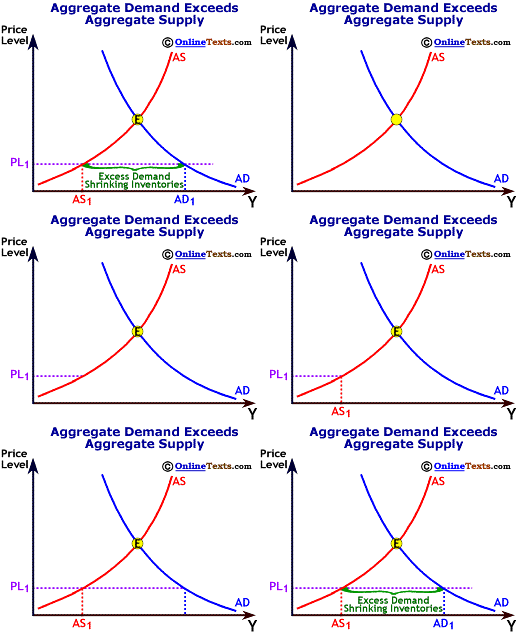 Suppose the economy is in disequilibrium. Let us consider first the case in which Aggregate Demand exceeds Aggregate Supply, or AD > AS. Demand for goods and services is greater than the production of goods and services. As demand outpaces supply, firms see inventories declining unexpectedly and they respond by increasing output and prices until equilibrium is reached. As the price level rises, aggregate demand declines due to the wealth and international trade effects, and aggregate supply rises due to firms' potential for larger profits. This scenario is illustrated in the figure titled "Aggregate Demand Exceeds Aggregate Supply."
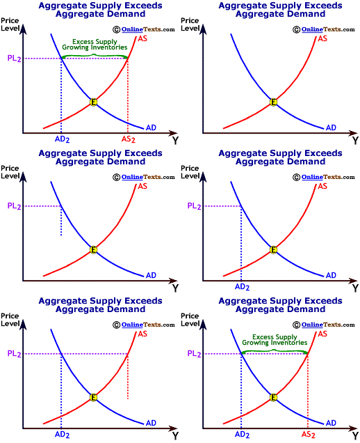 The alternative scenario, illustrated in the figure titled "Aggregate Supply Exceeds Aggregate Demand," occurs when the price level is too high such that Aggregate Demand is less than Aggregate Supply, or AD < AS. Demand for goods and services is less than production of goods and services, and firms see inventories increasing unexpectedly. They respond by decreasing production and prices. As the price level falls, Aggregate Demand increases and Aggregate Supply decreases. Again, the economy tends towards equilibrium.

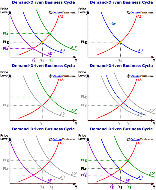
Having explained the theoretical framework, we are now ready to explain business cycle behavior using the Aggregate Demand/Aggregate Supply model. Generally, economic expansions and contractions are driven by shifts in the Aggregate Demand or Aggregate Supply curves. In more "typical" business cycles, fluctuations in Aggregate Demand generate movements in output and price. As the figure labeled "Demand-Driven Business Cycle" illustrates, rightward shifts in the Aggregate Demand curve increase both the price level and the level of output. In other words, in a typical business cycle expansion, economic growth is accompanied by rising prices. Conversely, leftward shifts in the Aggregate Demand curve decrease both the price level and the level of output. Demand-driven contractions, therefore, lead to declining levels of output and prices. In the real world, the price level does not actually fall but inflation decreases. Recessions and lower inflation rates tend to go together.

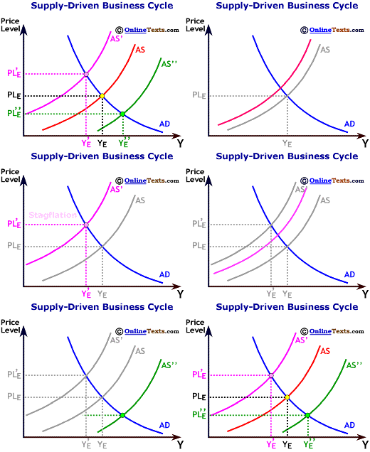
Supply-driven business cycles are caused by shifts in the Aggregate Supply curve. Aggregate supply shifts have played an increasingly important role since the 1970s. As the figure titled "Supply-Driven Business Cycle" illustrates, leftward shifts in the Aggregate Supply curve lead to both a rising price level and a contraction in output. These so-called supply shocks result in stagflation, the unfortunate combination of higher inflation and negative economic growth. The 1974-75 recession, the 1980 recession and the recession in 1990-91 were all precipitated by higher oil prices. Conversely, rightward shifts in the Aggregate Supply curve caused by, say, technological advances, decrease the price level and increase the level of output. Supply-side economics (see Chapter 12) is an attempt to shift the Aggregate Supply curve to the right, resulting in lower prices and higher levels of output. Supply-driven business cycles result in opposite movements in the price level and output.
|




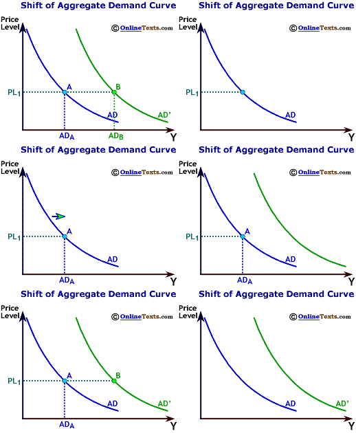


 A second factor that shifts the Aggregate Supply curve is a change in technology. As the Figure titled "Shift of Aggregate Supply Curve" illustrates, an increase in technology shifts the Aggregate Supply curve to the right. Technological progress influences the economy in a variety of ways. One channel is the introduction of entirely new goods and services. Just a few years ago an on-line textbook was not possible. Advances in the Internet, however, have enabled information to be delivered in a new way. Another way that technology influences the economy is through quality enhancements of products. In contrast to automobiles produced in the 1970s, today's cars are more dependable thanks to fuel injection systems and other automated components. Newer automobiles are also more fuel-efficient, and they have air bags and other safety features that older cars lack. A third way that technology is integrated into the economy is through cost-reducing innovations. The same product can be produced at a lower cost. First-generation computers used to take up areas the size of football fields. Today some hand-held calculators are just as powerful as those computer but the cost of producing a calculator is far less than the cost of producing an old-generation computer. Given the price level, cost-reducing technological advancements allow firms to increase production and boost profits.
 The short-run equilibrium occurs where the Aggregate Demand curve crosses the short-run Aggregate Supply curve. The intersection of Aggregate Demand and Aggregate Supply in the figure labeled "Short Run Equilibrium" determines both the price level and the equilibrium level of GDP in the economy. The level of output can be above or below potential output. For example, suppose that the economy produces $9 trillion of goods and services in the year 2005 and potential output is $8.5 trillion. As long as the demand for final goods and services is also $9 trillion, the economy is at a short-run equilibrium. Because supply and demand are equal, firms do not overproduce, which would lead to an unintended accumulation of inventories. Nor do firms underproduce, which would lead to an unintended depletion of inventories.
 The long-run equilibrium can only occur where the Aggregate Demand curve crosses the vertical Long Run Aggregate Supply curve because in the long run, equilibrium output must equal potential output where all resources are fully employed. This condition holds because in the short run, production input costs are held constant, but in the long run, input costs can vary. When output is above the potential level of output, there is pressure on wages to increase because workers are relatively scarce and employers bid up wages competing for the workers. As wages are bid up, the short-run Aggregate Supply curve shifts to the left until the equilibrium output is equal to potential output. This scenario is graphed in the figure labeled "Long Run Equilibrium."
 Suppose the economy is in disequilibrium. Let us consider first the case in which Aggregate Demand exceeds Aggregate Supply, or AD > AS. Demand for goods and services is greater than the production of goods and services. As demand outpaces supply, firms see inventories declining unexpectedly and they respond by increasing output and prices until equilibrium is reached. As the price level rises, aggregate demand declines due to the wealth and international trade effects, and aggregate supply rises due to firms' potential for larger profits. This scenario is illustrated in the figure titled "Aggregate Demand Exceeds Aggregate Supply."
 The alternative scenario, illustrated in the figure titled "Aggregate Supply Exceeds Aggregate Demand," occurs when the price level is too high such that Aggregate Demand is less than Aggregate Supply, or AD < AS. Demand for goods and services is less than production of goods and services, and firms see inventories increasing unexpectedly. They respond by decreasing production and prices. As the price level falls, Aggregate Demand increases and Aggregate Supply decreases. Again, the economy tends towards equilibrium.
