Chapter Eleven: Lecture Notes -- The Output Multiplier


When an autonomous component of Aggregate Demand changes, equilibrium output (Y) will change. The change in output will be even larger than the initial change in Aggregate Demand. This result for the change in Y to be greater than the initial change in Aggregate Demand is known as the multiplier effect. For example, if the marginal propensity to consume (MPC) is 0.80 and autonomous investment increases by $200, equilibrium output will ultimately change by $1,000, not $200!


The simple output multiplier = 1/(1-MPC).

Calculating the Size of the Multiplier Effect

The size of the multiplier effect is given by:
where the (simple) output multiplier is defined as 1/(1-MPC). For example, with an MPC of 0.80, the simple output multiplier is 1/(1-0.80) = 5, so the $200 initial increase in investment ultimately increases output by 5 x $200 = $1,000.

The simple output multiplier assumes there are no proportional taxes, all expenditures are for domestically produced goods and services, and the price level is fixed.


Income-induced consumption is the key to understanding the output multiplier.

How and Why the Multiplier Works

Consumption is based primarily on disposable income. When Aggregate Demand rises, output and hence income rise. The rise in income allows people to consume more goods and services. This is called "income-induced" consumption and it raises Aggregate Demand even more.

TABLE 1
Round Initial Change
in Investment
Change in
Output
Change in
Consumption
1 $100 $100.00 $80.00
2 0 $80.00 $64.00
3 0 $64.00 $51.20
4 0 $51.20 $40.96
5 0 $40.96 $32.77
6 0 $32.77 $26.21
7 0 $26.21 $20.97
8 0 $20.97 $16.78
9 0 $16.78 $13.42
10 to inf. 0 $67.11 $53.69
Totals $100 $500 $400.00

Let's work through an example of the multiplier process. Suppose the MPC is 0.80. A University decides to build a new residence hall worth $100 million. Construction workers earn $100 million in income, and they spend 80 percent--or $80 million--dining out, going to the movies, shopping, and buying new cars. The increased spending of $80 million becomes income to the owners and employees of the restaurants, movie theatres, shopping malls, and car dealers. In turn, these people spend 80 percent of the new $80 million, or $64 million, on other goods and services. The $64 million becomes income to others in the community, and the process continues. Table 1 shows the impact of the multiplier through various rounds. When all the effects are totaled up, output will increase by $500 million because the value of the output multiplier is equal to 1/(1-0.8) = 5. Remember that the initial increase in Aggregate Demand for the new residence hall was just $100 million.


Proportional taxes reduce the size of the multiplier.

The Output Multiplier with Proportional Taxes

One by one, we will relax the assumptions we made in calculating the simple output multiplier. Let us start by introducing proportional taxes. A proportional tax is a tax that varies with the level of income. An example is the income tax. If income is taxed at a 20 percent rate, then t = 0.20, where t is the tax rate. Tax revenue (T) is the total revenue collected from the tax. It is computed by the formula:

    T = t × Y.

The formula for the output multiplier when proportional taxes are present, is:

If MPC = 0.80, and t = 0.25, then the output multiplier is

1/(1-0.80(1-0.25)) = 1/(1-0.6) = 1/0.4 = 2.5.

TABLE 2
Round Initial Change
in Investment
Change in
Output
Change in
Consumption
1 $100 $100.00 $60.00
2 0 $60.00 $36.00
3 0 $36.00 $21.60
4 0 $21.60 $12.96
5 0 $12.96 $7.78
6 0 $7.78 $4.67
7 0 $4.67 $2.80
8 0 $2.80 $1.68
9 0 $1.68 $1.01
10 to inf. 0 $2.52 $1.51
Totals $100 $250 $150

Proportional taxes reduce the size of the multiplier because when there is, say, $100 of new Aggregate Demand, an MPC of 0.8, and a 25 percent tax rate, output increases in the first round by $100 but disposable income only goes up by DI = Y - T = $100 - (.25 × 100) = $75. Consumers will spend 80 percent of that $75, or $60 in the first round. Taxes diminish induced consumption, which in turn diminishes the impact on output in the next round. Total output now changes by only $250, not $500. Table 2 illustrates the impact of the tax rate on the multiplier effect of the $100 million investment in the residence hall.


The propensity to import tends to lower the multiplier effect.

The Output Multiplier with Imports

When domestic income rises, consumers wish to purchase more goods and services. Some of the things they wish to consume are imports. When income rises, demand for foreign goods and services also rises. This lowers demand for U.S. goods & services and thus dampens the multiplier effect. We define the marginal propensity to import (MPI) as the change in imports divided by the change in disposable income. For example, suppose the MPI = 0.05. If disposable income (DI) rises by $100, imports will rise by $5.

Assuming no proportional taxes but including imports, the output multiplier formula is:

With an MPC = 0.8 and MPI = 0.05, the value of the output multiplier is
1/(1 - 0.8 + 0.05) = 1/0.25 = 4.
Like taxes, the propensity to import tends to lower the multiplier effect because demand for domestically produced final goods and services falls.


An Interactive Example

Below are two interactive tables that compute the value of the output multiplier and display the impact of the multiplier through ten rounds. Enter in values for the MPC (it must be between 0 and 1), the tax rate (between 0 and 100), and the initial change in Aggregate Demand. Then click the "Compute" button. The "Reset" button resets all the numbers to their default values.

Output Multiplier

MPC (between 0 and 1):
Tax rate (as %):
Initial Change in AD:
Multiplier:

Rounds of the Multiplier

RoundInitial Change
in AD
Change
in Y
Induced change
in Consumption
1
2
3
4
5
6
7
8
9
10
Total


A rising price level also tends to reduce the value of the multiplier.

The Output Multiplier with Price Level Changes

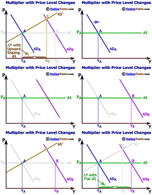
Multiplier is smaller if price level varies Just for this section, we will relax the assumption of fixed prices. The figure titled "Multiplier with Price Level Changes" assumes that the Aggregate Supply curve is upward sloping instead of perfectly horizontal. When the Aggregate Demand curve shifts and the Aggregate Supply curve is upward sloping, the multiplier effect is smaller. The economy moves from point A to point C, instead of going to point B when the Aggregate Supply curve is horizontal. The smaller effect results because Aggregate Demand is partially dampened as the price level rises. With an upward sloping Aggregate Supply curve, the impact of an increase in Aggregate Demand goes towards higher output and prices. In the extreme case of a perfectly vertical Aggregate Supply curve, the output multiplier is zero.


Temporary expenditures flow through the economy, but they do not have a permanent effect on the equilibrium level of output.

The Multiplier Effect and a Temporary Change in Aggregate Demand

Recall that the multiplier effect is calculated by:

The dynamic impact of the multiplier depends upon whether the change in Aggregate Demand is temporary (a one-time expenditure), or permanent (a permanent period after period increase in Aggregate Demand). For example, if a government repairs a road, the injection into the economy is temporary. When the road is finished, the new government injections into the economy stop. The expenditures on the road will flow through the economy, but they will not continue indefinitely.

On the other hand, the construction of a new public school building or a new jail is more permanent. The government expenditures continue even after construction of the building is completed. New jobs for teachers, staff, and administrators will be created and the government must continue to pay income to these workers year after year. First, we examine the multiplier effect when the initial injection of Aggregate Demand is temporary.
Temporary Shift of AD Curve

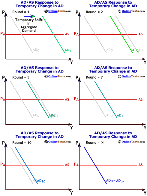
Suppose the government spends $100 to repair an existing road, injecting $100 temporarily into the economy. The multiplier effect occurs over a period of time. Assuming no taxes or imports and an MPC of 0.8, an increase in government expenditures of $100 ultimately increases output by a total of $500, but the increase in output will not occur all at once. As the figure titled "AD/AS Response to Temporary Change in AD" illustrates, initially, AD0 and AS intersect. The one-time $100 increase in Government Expenditures in round 1 shifts the Aggregate Demand curve to the right (AD1). After this expenditure, Government Expenditures decline by $100 because the road repair project is completed. The increase in income from the road improvement increases consumption and output in round 2, but only by 0.8 × $100,or $80. So output is actually $20 lower compared with the previous round. The intersection of AD2 and AS gives the level of output in round 2. The process continues in round 3, and again in round 4. Each time the Aggregate Demand curve shifts to the left. Eventually, the Aggregate Demand curve will exactly overlie the original AD0curve, and the multiplier effect will be completed. A useful analogy is to think of a stone thrown into a still lake. The initial impact makes the biggest splash and then the impact ripples through the water in successively smaller waves. Eventually, the water returns to its initial peaceful condition.
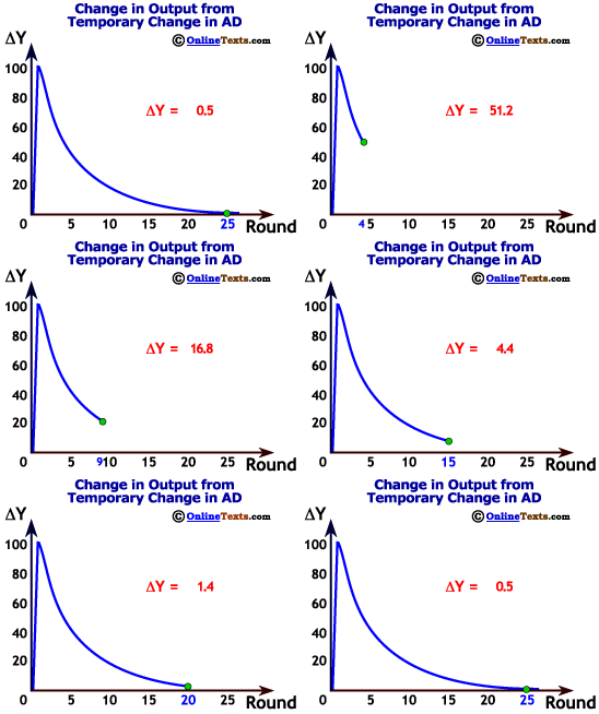
Change in output from a temporary increase in AD

Because of the road repair expenditures, equilibrium output rises, but the impact dampens out over time. The figure titled "Change in Output from Temporary Change in AD" shows the change in equilibrium output in each round. Notice that the change in equilibrium output asymptotically returns to zero.


Permanent expenditures have a lasting effect on the equilibrium level of output.

The Multiplier Effect and a Permanent Change in Aggregate Demand

Permanent Change In AD

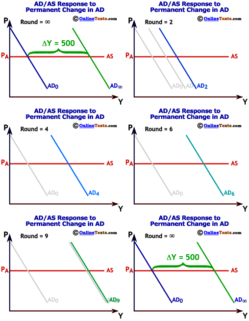
If the government(or any private investor) funds an on-going project like financing a school, the impact is much larger than that of a temporary spending increase. Suppose for simplicity that the government spends $100 to construct a new school and then spends $100 each year to operate the school. The government is injecting $100 into the economy permanently.


Output Change due to Permanent Change in AD

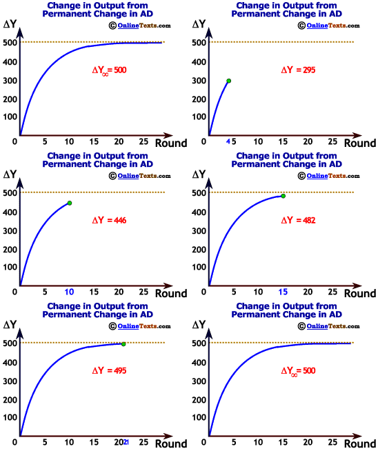
As the figure titled "AD/AS Response to Permanent Change in AD" illustrates, in the first round, output increases by $100 due to the initial change in government spending. The higher output and, hence, higher income induces $80 more consumption spending (assuming an MPC of 0.8, and no imports or taxes). If the government expenditure is permanent, total output rises in the second round by $180 ($100 of government expenditures plus $80 for the induced consumption). In the third round, consumption increases again by an additional $64 ($80 x 0.8), so output increases by $100 + $80 + $64,or $224. The process continues with each successive increase in output becoming smaller and smaller until the incremental change in output is zero. However, the overall equilibrium level of output in the community will be $500 (5 x $100) higher than before the school was built and operated. The cumulative impact on the equilibrium level of output is illustrated in the figure titled "Change in Output from Permanent Change in AD."


Conclusion

The multiplier almost seems magical, in that the economy is getting something for nothing. Not so. The multiplier process is the result of numerous businesses and individuals increasing their production activities to take advantage of potential profit opportunities.

Although the multiplier process can be a powerful force of economic expansion or contraction, we must keep in mind that the process occurs primarily in the short run. Imagine a city with a fully employed labor force that builds a new high school out in the suburbs. The spending for the high school creates multiplier effects as teachers and staff earn income and then spend that income on other things in the community. If the teachers and staff at the new high school, however, came from a city high school which was closed, then the overall multiplier effect on the region is much smaller (and may even be zero) because income in the community where the school was closed is less. The multiplier effect has its greatest impact when idle resources exist.


Copyright © 1995-2006 OnlineTexts.com - All Rights Reserved