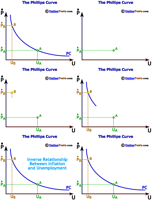
The Phillips curve illustrates the inverse relationship between inflation and unemployment. |
Chapter Sixteen: Lecture Notes -- The Phillips Curve
The Phillips curve is a graph illustrating the relationship between inflation and the unemployment rate. The Phillips curve is a dynamic representation of the economy; it shows how quickly prices are rising through time for a given rate of unemployment. The relationship between inflation and unemployment depends upon the time frame. The short-run Phillips curve, illustrated in the figure titled "The Phillips Curve", shows that the relationship between the inflation rate () and unemployment is negative. When inflation rises, unemployment falls and vice versa.
This relationship helps to explain the adage "there is no good news in economics." When one side of the economy is doing well, the other side tends to do poorly. For example, if unemployment is low, inflation tends to be relatively high. Journalists often focus on the parts of the economy doing poorly. Because of the relationship represented in the Phillips curve, economists in the late 1950s and 1960s thought that all the Federal Reserve or government had to do was to pick the point on the short-run Phillips curve that they wanted the economy to be on. If they wanted to have less unemployment and operate, for example, at point B on the graph instead of point A, then they had to live with more inflation. This simplistic notion turned out to be false in the 1970s, forcing economists to rethink the whole notion of the Phillips curve.
|
A significant difference exists between the long-run and short-run Phillips curves. |
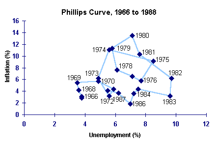
Breakdown of the Short-Run Phillips CurveIn the 1970s and early 1980s the short-run relationship between inflation and unemployment seemed to break down. As the figure titled "Phillips Curve, 1966 to 1988" illustrates, inflation was often high even while unemployment was high. Between 1973 and 1974 and again between 1979 and 1980, both inflation and unemployment increased. Rather than approximating a straight line, the Phillips curve seemed to spiral clockwise. Standard Keynesian economics could not explain why the Phillips curve had gone haywire. Did the economy fundamentally change or was there something missing from the theory that needed to be incorporated?Economists were able to salvage the Phillips curve by realizing that a significant difference exists between the short-run and long-run relationship between inflation and unemployment. |
|
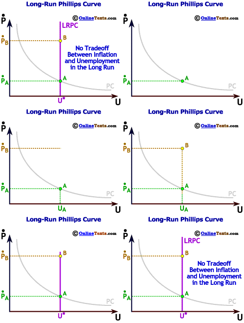
The long-run Phillips curve is vertical, suggesting that there is no tradeoff between unemployment and inflation. |
The Long-Run Phillips Curve
Most economists now agree that in the long run there is no tradeoff between inflation and unemployment. Since in the long run the economy produces at potential output (YP)--the point at which the unemployment rate is at the natural rate--the long-run Phillips curve is simply a vertical line at the natural rate of unemployment, U*. As the figure titled "Long-Run Phillips Curve" illustrates, any level of inflation is consistent with the natural rate of unemployment. For example, at point A the unemployment rate is at U* and the inflation rate is A. At point B, the unemployment rate is |
..... |
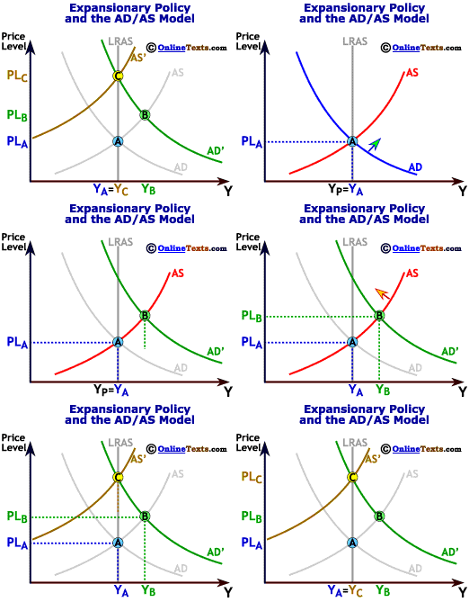
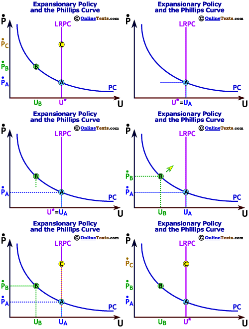
Aggregate Demand Shifts and the Phillips CurveWe can "explain" both the short-run and long-run Phillips curves by using the Aggregate Demand/Aggregate Supply model that we developed in Chapter 8. First, let us look at the short-run relationship between inflation and unemployment. We begin at point A in the left-hand chart titled "Expansionary Policy and the AD/AS Model", where the economy is at potential output YP. Because the economy is at potential output, the unemployment rate in the Phillips curve--plotted in the right-hand chart titled "Expansionary Policy and the Phillips Curve") is U*, the natural rate of unemployment, and the inflation rate is A. |
|
Any factor that shifts the Aggregate Demand curve moves the economy along the short-run Phillips curve. |
Suppose that the Aggregate Demand curve shifts to the right for any reason, say the result of expansionary fiscal or monetary policy. This expansionary policy increases the price level (from PLA to PLB) and output (from YA to YB)in the Aggregate Demand/Aggregate Supply model such that the economy moves from point A to point B in the left-hand figure. In the Phillips curve plotted in the right-hand figure, the higher price level corresponds with higher inflation, and the higher level of output means that more people are working, so unemployment falls. The economy moves along the Phillips curve in the right-hand chart from point A to point B.
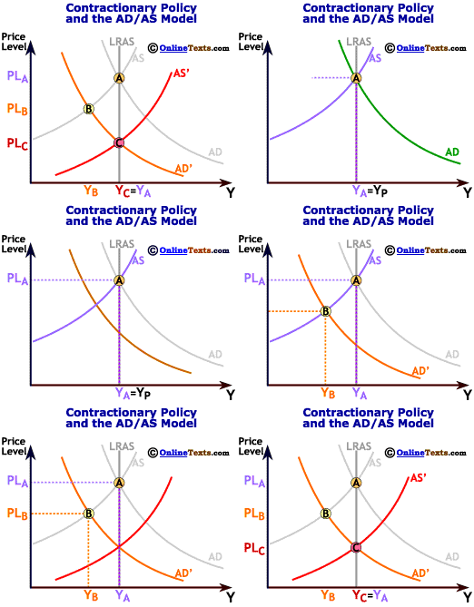
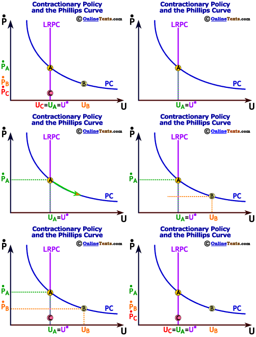
This story leads to an important generalization. Any factor that shifts the Aggregate Demand curve, moves the economy along the short-run Phillips curve. When the Aggregate Demand curve shifts to the right, the economy moves up and to the left on the short-run Phillips curve because the price level rises corresponding with a rise in inflation, while the level of output increases, which decreases unemployment. Conversely, when the Aggregate Demand curve shifts to the left, the economy moves down and to the right on the short-run Phillips curve. Point B in both charts cannot be a long-run equilibrium since the economy is not at potential output nor at full employment. The high level of output (relative to potential output) eventually increases wages as workers become more difficult to find and employ. This increase in input costs shifts to the left the Aggregate Supply curve in the left-hand chart to point C. As the price level rises to PLC, the level of output returns to YP, so the economy's level of unemployment must again be U*. In the right-hand chart of the Phillips curve, the economy moves from point B to point C, reflecting the higher inflation and the higher unemployment. Point C in both charts is a long-run equilibrium. Observe points A and C in the right-hand chart. The unemployment rate is identical but the rate of inflation at point C is much higher than at point A. This transition demonstrates the principle behind long-run Phillips curve such that in the long-run there is no tradeoff between inflation and unemployment. The figures below titled "Contractionary Policy and the AD/AS Model" and "Contractionary Policy and the Phillips Curve"illustrate exactly the same concepts, but they describe the economy's response to a leftward shift in the Aggregate Demand curve. Both charts begin at point A, points in which the economy is in a long-run equilibrium. The leftward shift of the Aggregate Demand curve decreases the price level and output, moving the short-run equilibrium to point B in the left-hand chart. As a consequence, the economy experiences lower inflation and higher unemployment, represented by the movement from point A point B in the right-hand chart. In the long run, the Aggregate Supply curve shifts to the left in the left-hand chart as wages decline in response to the excess unemployment. Eventually the economy moves to point C, again a long-run equilibrium. Relative to point A, the economy has the same level of output but a lower price level (PLC versus PLA). We illustrate this scenario by a move along the Phillips curve from point B to point C in the right-hand chart. Points A and C each show the economy at full employment (U*), however, point C has a lower rate of inflation than point A. |
|
................ |
The Role of ExpectationsThe short-run tradeoff between inflation and unemployment is thought to work because people have an idea of what inflation expectations are going to be, and those expectations change slowly. When the Aggregate Demand curve shifts to the right, prices and output increase. This shift increases inflation and lowers unemployment. Firms respond to this situation by attempting to hire workers. Workers view the wage offered as "good" since they do not expect that prices will rise also. But in the long-run, workers learn that inflation has risen and they are no longer happy with their wage, so they increase their inflation expectations. Workers demand larger increases in wages which forces firms to lay off some workers until the economy arrives back at the natural rate of unemployment. We can express the Phillips curve as an equation in the following manner:
where is the expected rate of inflation based upon inflation expectations, b is a constant greater than zero reflecting the inverse relationship between inflation and unemployment, U is the current unemployment rate, and U* is the natural rate of unemployment.
For example, suppose that =3%, b=0.5, U*=5% and U=4.0%. From these parameters, we know that
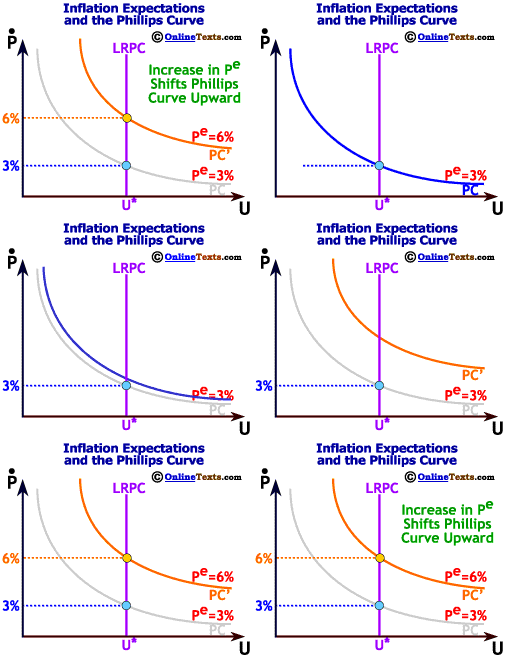
Note that in the long-run U* = U, so The long-run Phillips curve equation suggests that the inflation rate is entirely determined by inflation expectations. As the figure titled "Inflation Expectations and the Phillips Curve" illustrates, when inflation expectations rise, the Phillips curve shifts upward. In particular, when inflation expectations rise from 3 percent to 6 percent, the short-run Phillips curve shifts upward until the inflation rate is 6 percent when the economy is at the natural rate of unemployment. Now we can understand the differences between the short-run and long-run Phillips curves. In the short run, an increase in Aggregate Demand does move the economy up to the left along the short-run Phillips curve. Output and inflation increase while unemployment decreases. Over the longer term, however, inflation expectations increase and workers no longer work the extra hours because they realize that real wages have not increased with the increase in prices. Output returns to the same level as before but inflation is higher because it is built into the system in terms of higher inflation expectations. The long run Phillips curve, therefore, is vertical. |
................ |
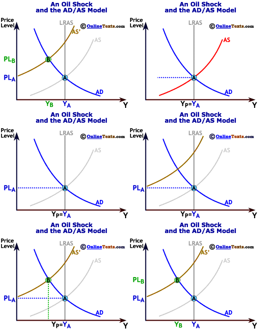
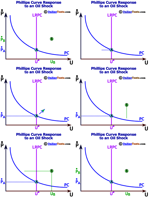
Shifts in the AS CurveWhen the Aggregate Supply curve shifts, we can get very different results in the Phillips curve. For example, let us take the case of an oil shock. As we see in the left-hand chart titled "An Oil Shock and the AD/AS Model", an oil shock shifts the Aggregate Supply curve to the left and the result is stagflation--a rise in both inflation and unemployment. On the Phillips curve plotted in the right-hand chart titled "Phillips Curve Response to an Oil Shock", the oil shock produces a movement to the northeast of point A as both unemployment and inflation increase. |
|
................ |
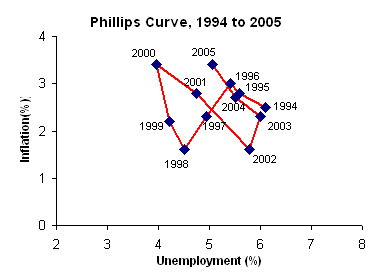
Often in response to a severe negative supply shock (such as an oil shock), inflation expectations rise quickly and the short-run Phillips curve shifts upward. Even after the economy's move northeast on the Phillips curve, policy makers are stuck with the short-run tradeoff between inflation and unemployment. If policy is contractionary to lower inflation, unemployment will rise even further. If policy is expansionary to eliminate the excess unemployment, inflation will rise even higher. In the long run the economy will end up back on the long-run Phillips curve with a high rate of inflation. What should the Federal Reserve do with regards to monetary policy in this scenario? In the late 1970s the Federal Reserve faced just this decision. There is no good alternative for the Fed. Either they alleviate unemployment and live with higher inflation, or they cause a large recession and eliminate high inflation. The Fed opted for the latter which led to a deep recession in the United States. Unemployment peaked above 10 percent in the early 1982. However, in the long run (about six years after the 1982 recession), the economy had 3 to 4 percent inflation and was back to the natural rate of unemployment. The overall point is that a leftward shift in the Aggregate Supply curve does not move the economy along the short-run Phillips curve, but it moves the economy to a point that is northeast of its present state. If inflation expectations increase, the Phillips curve shifts upward. Of course, a positive supply shock can shift the Phillips curve down as inflation expectations fall. Once either of these things happens however, the policy makers are still faced with the same short-run tradeoff between inflation and unemployment. Is the Phillips Curve Dead?Despite being reconstructed in the 1970s, the Phillips curve threw economists for a loop again in the 1990s. During much of the 1990s, the Phillips curve relationship was suspiciously absent, as the figure titled "Phillips Curve, 1994 to 2005"illustrates. The economy's rate of unemployment fell, for example, from 7.8 percent in 1992 to 4.0 percent in 1999. Despite this decline, inflation did not rise much. In fact, in 1997 and 1998 inflation fell even further relative to previous years. Economists are not exactly sure why this happened, although lower oil and food costs played a significant role.Another important factor explaining the odd behavior of the Phillips curve in the 1990s is labor productivity, or output per labor hour. (See Chapter 18, Economic Growth and Productivity.) Recall that one reason for the short-run trade-off between inflation and unemployment is that when unemployment declines, wage pressures increase, driving up prices. If productivity growth is high, however, firms can pay workers higher wages and still keep price increases modest becuase those workers are more productive. Productivity did begin to increase in the mid-1990s, and it has remained high through 2003. The surge in productivity is perhaps the key reason why wages and, hence, prices have not risen with the decline in unempoyment rates in the 1990s.
Similar to the 1970s, many economists are seriously questioning the usefulness of even the modified inflation-expectations version of the Phillips curve. The events of the 1990s indicate that, at the very least, the Phillips curve is not a reliable tool to forecast inflation. Indeed, some economists are discounting the supposed short-run relationship between inflation and unemployment altogether, arguing that the relationship is too volatile to be a reliable guide. No new consensus has emerged as of yet. Although many economists agree that the forecasting power of the Phillips curve is limited at best, they continue to believe that the Phillips curve does a fairly good job at explaining economic behavior after the fact.
|
Useful Web Resources
|
Copyright © 1995-2006 OnlineTexts.com - All Rights Reserved |